Probing Lunar Swirls.
Bright, sinuous markings with no topography of their own — and a transformer trained to read twelve maps of the Moon at once, then probed to ask which story about them the data actually supports.
Tom Sander, Kay Wohlfarth, Mirza Arnaut, Marcel Hess & Christian Wöhler · TU Dortmund
A mystery written in albedo
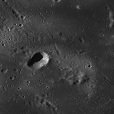
Lunar swirls — Reiner Gamma is the classic example — are bright, looping markings that have no topographic or stratigraphic expression: they sit flat on the surface, often draped over crater and mare alike. They tend to coincide with crustal magnetic anomalies, though exceptions like the swirls in Mare Moscoviense complicate a purely magnetic story. After decades of observation their origin is still unsettled. Three families of hypotheses compete — and, crucially, each predicts a different fingerprint in how the surface's physical properties couple together.
Solar-wind shielding
A local magnetic field deflects the solar wind, slowing space weathering. The surface stays optically immature — maturation retardation.
Predicts
Composition–reflectance link is preserved inside swirls.
Cometary impact
A comet coma scours and thermally alters the regolith, leaving a swept, compacted surface behind.
Predicts
Thermal emission couples more strongly inside swirls.
Dust transport
Electrostatic sorting moves fine, bright dust across the surface, rearranging the upper regolith structure.
Predicts
Radar roughness couples more strongly inside swirls.
The idea of this work is not to predict swirls, but to turn a trained model into a diagnostic instrument: measure which signals depend on which, inside the swirls versus outside, and see whose fingerprint the Moon is actually wearing. We return to these three cards at the end — with verdicts.
Twelve ways of seeing one place
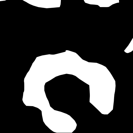
Every swirl site is imaged by many instruments at once, each co-registered to the same 300-pixel-per-degree grid: an optical mosaic, radar backscatter, elemental abundance maps, spectral band-depth indices, thermal brightness temperature, and its own latitude/longitude. Below is a single site seen through nine of these maps — flip between them, and toggle the swirl boundary to see where the bright markings actually fall.
WAC reflectance
LRO Wide Angle Camera reflectance — the visible brightness that makes swirls stand out in the first place.
The boundary is the Denevi et al. shapefile catalog, rasterized to the same grid and used as the supervised label.
An atlas of every known swirl
The 56 sites cluster into eight complexes spread across the near and far side. Seven complexes are used for training; the Rumfold-T complex is held out entirely for testing, so the model is always judged on geography it has never seen. Hover a site for its coordinates. Switch to cross-modal coupling to overlay the spatially-resolved probe: each dot is one 128-pixel tile, coloured by how much the optical channel leans on titanium there.
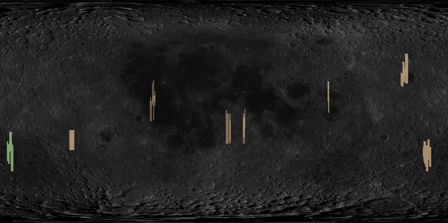
56 sites across 8 complexes. Longitude 0–360° is remapped to ±180° to match the mosaic.
Legend
One model, twelve tongues
Every image-like modality gets its own VQ-VAE tokenizer (Cosmos-style): an 8×8 patch becomes one discrete token drawn from that modality's codebook, giving 256 tokens per 128-pixel tile. The odd one out is position — latitude and longitude are handled by a structure-aware regex tokenizer that treats each digit, degree marker and hemisphere letter as its own semantic unit. All the token sequences are concatenated, a random subset is masked, and a shared transformer encoder–decoder reconstructs the hidden tokens.
The coordinate tokenizer
Move a swirl's position and watch the token string rebuild — a 64-symbol vocabulary, no free-form text.
The masking strategy
Twelve modalities, one shared sequence. Filled cells are shown to the encoder; hollow cells are masked and must be predicted.
Tokenizer & model configuration
| Modality | Codebook |
|---|---|
| WAC · sc-pol · op-pol | 2048 / 1536 / 1536 |
| ibd1 · bt | 1024 / 1536 |
| titan · iron · aluminum · calcium | 1024 each |
| plagioclase · pyroxene | 1024 each |
| position (regex) | 64 |
| Hyperparameter | Value |
|---|---|
| Encoder / decoder depth | 6 + 6 |
| Hidden dim · heads | 132 · 6 |
| Patch · tokens/tile | 8×8 · 256 |
| Optimizer | AdamW, cosine decay |
| Loss | token-normalized cross-entropy |
Can it reconstruct the Moon?
Before the model can be trusted as a probe, it has to actually reconstruct the held-out data. Pick a modality and drag the divider to wipe between the model's prediction and the ground truth. Smooth elemental and radar maps come back almost perfectly; the visually busy optical mosaic and the fine-grained mineral maps are intrinsically harder — high spatial frequency, not a failure of the model.
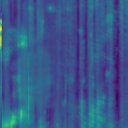
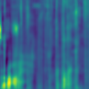
Titanium reconstructs almost losslessly (SSIM 0.998) — smooth elemental maps sit comfortably inside the tokenizer's discrete bottleneck.
Full reconstruction tables
| Full-model reconstruction, held-out test set (Table 2) | |||
|---|---|---|---|
| Modality | SSIM ↑ | PSNR ↑ | RMSE ↓ |
| aluminum | 0.9864 | 44.11 | 0.0065 |
| brightness_temperature | 0.9055 | 18.56 | 20.98 |
| calcium | 0.9449 | 35.65 | 0.0014 |
| ibd1 | 0.9623 | 40.89 | 6.856 |
| iron | 0.9971 | 53.54 | 0.0182 |
| op-pol | 0.9663 | 41.60 | 0.0190 |
| plagioclase | 0.6973 | 22.67 | 6.340 |
| pyroxene | 0.6096 | 21.88 | 4.242 |
| sc-pol | 0.9770 | 44.00 | 0.0123 |
| titan | 0.9981 | 54.01 | 0.0155 |
| wac | 0.5965 | 19.54 | 0.0148 |
The position channel is different. Encoded as text, it recovers the structure of a coordinate string (normalized Levenshtein 0.405) but almost never the exact values (parse rate ≈ 0, great-circle error ~1866 km). That is physically expected: local mineralogy and radar roughness carry no global geolocation signature, so position acts as a contextual anchor, not a decodable coordinate — the same conclusion the latent-space analysis reaches independently.
Which signals actually matter
Now the probing begins. Two ablations ask complementary questions of a linear classifier trained to trace swirl boundaries. Leave-One-Out removes each modality and measures how far F1 drops — its necessity. Leave-One-In keeps only that modality (plus position) and measures how far it beats the spatial baseline — its sufficiency. A modality matters most where it cannot be substituted by the others.
Necessity (LOO F1 drop, Δ). Baseline F1 with every modality present is 0.492.
Inside the latent space
Two more probes read the model's internals. Attention shows which source modality the transformer routes to when predicting each target. Representational similarity compares the geometry of the learned features pairwise. In both, the interesting cells are the outliers — and one stands out everywhere: position sits apart from every physical channel.
Attention routing
Rows are the target being predicted, columns the source being read. The single hottest route is optical reflectance attending to titanium (mass 0.34); pyroxene leans hard on iron (0.28). The position column stays cold everywhere — the model barely consults coordinates to reconstruct physics.
The verdict
The decisive experiment extends the ablations into space: for each hypothesis target, withhold a whole group of inputs and measure how much more the model relies on it inside swirls than outside. A positive bar means the coupling strengthens inside the swirl — the fingerprint that hypothesis predicts. Only one target lights up positive.
Δ = ⟨deviation⟩in-swirl − ⟨deviation⟩off-swirl, per withheld modality group. Targets: optical (wac), thermal (bt), radar roughness (sc-pol). The bt × phys-thermal bar is absent by design — brightness temperature is the thermophysical group.
Maturation retardation
Optical reflectance depends more on composition inside swirls (Δ = +0.10). Where weathering is slowed, the link between mineralogy and brightness survives — exactly this prediction.
Cometary / thermophysical
Brightness temperature couples less inside swirls (Δ = −0.40), not more. No sign of a thermally distinct, swept surface.
Dust transport
Radar roughness coupling is negative across every group — no evidence of the reorganized upper regolith this scenario needs.
An honest caveat. This is not a refutation of the alternatives — orbital data cannot resolve subsurface magnetic geometry, and absence of evidence at 300 px/deg is not evidence of absence. The claim is narrower and cleaner: within current orbital archives, only the optical–compositional signature carries the asymmetry maturation retardation predicts. The 56 sites also span just 8 complexes, so "population-level" means the catalogued swirls, not a statistically independent sample. Settling the mechanism will need in-situ measurement — the kind the upcoming Lunar Vertex mission is designed for.
Paper & code
Computers & Geosciences
The manuscript “Probing Lunar Swirls with a Multimodal Transformer” is currently under peer review. The full source — model, tokenizers and the probing protocol — is public on GitHub; every figure and number on this page is drawn directly from the submitted manuscript.
Swirl-MAE on GitHubThe predecessor
The any-to-any multimodal transformer this probing framework builds on — reconstructing elevation, normals and albedo of the Moon.
Related project
Anomaly detection at the Apollo sites, on the same Shape-from-Shading data pipeline.
Architecture lineage: the framework adapts masked multimodal modelling (MultiMAE / 4M, Bachmann & Mizrahi et al.) with Cosmos-style VQ-VAE tokenizers to heterogeneous lunar remote sensing.